Project 3: Performance Programming
Project 2.2 Project 3
Introduction
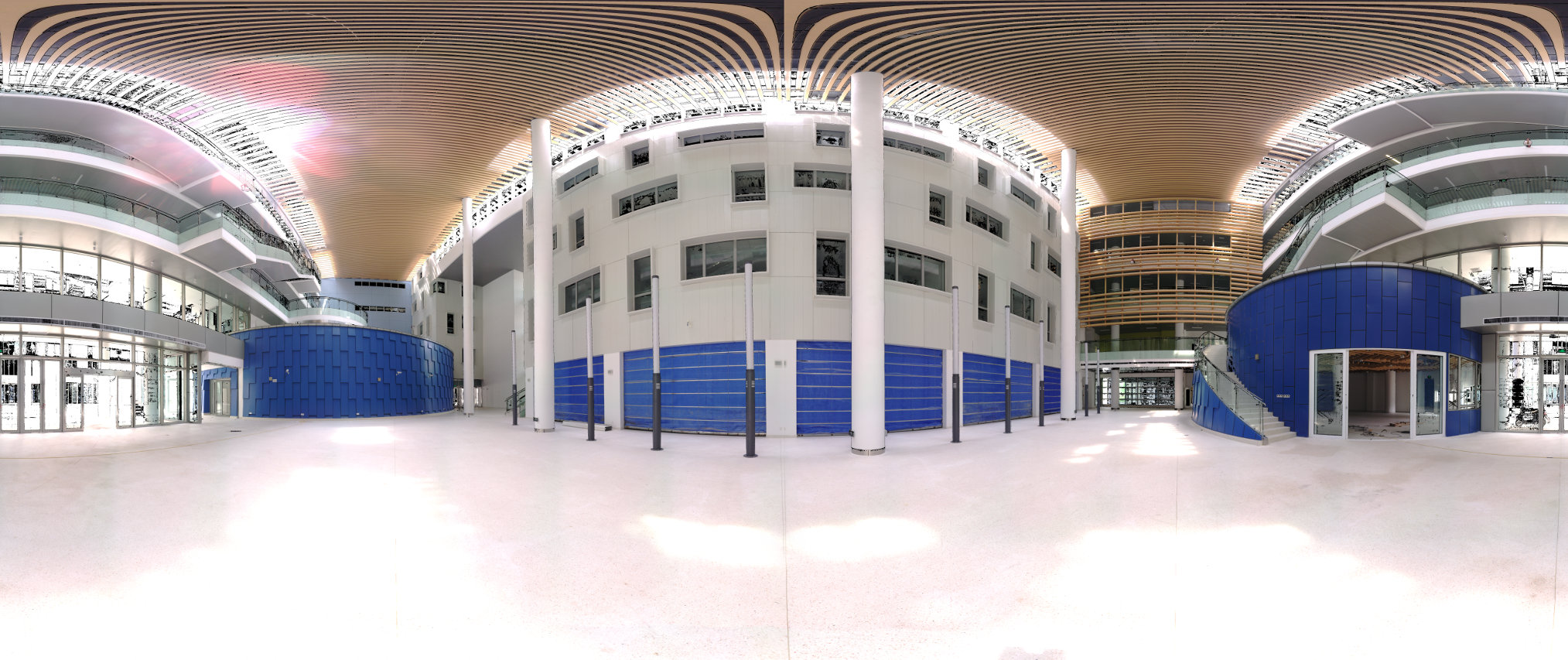
SIST has a 3D laser scanner (Faro Focus 3D X330) that can also gather the color of the 3D points. More information on 3D scanning can be found on Wikipedia.For this project we want to post-process such scans. We will be working with a scan taken in the lobby of the new SIST building (see Fig. 1). This scan has a resolution of 20265 x 8533 pixel - that are about 173 million pixel. A video showing this and 7 more scans in the lobby is available here (299MiB).
Since this is a 3D scan we not only get the colors of the pixel but also the distance of that pixel from the camera. For this project, this information is encoded in a separate file which first saves the width and height of the depth image as 32bit unsigned integers (little-endian) followed by the depth information as floats in meter. The file can be downloaded below.
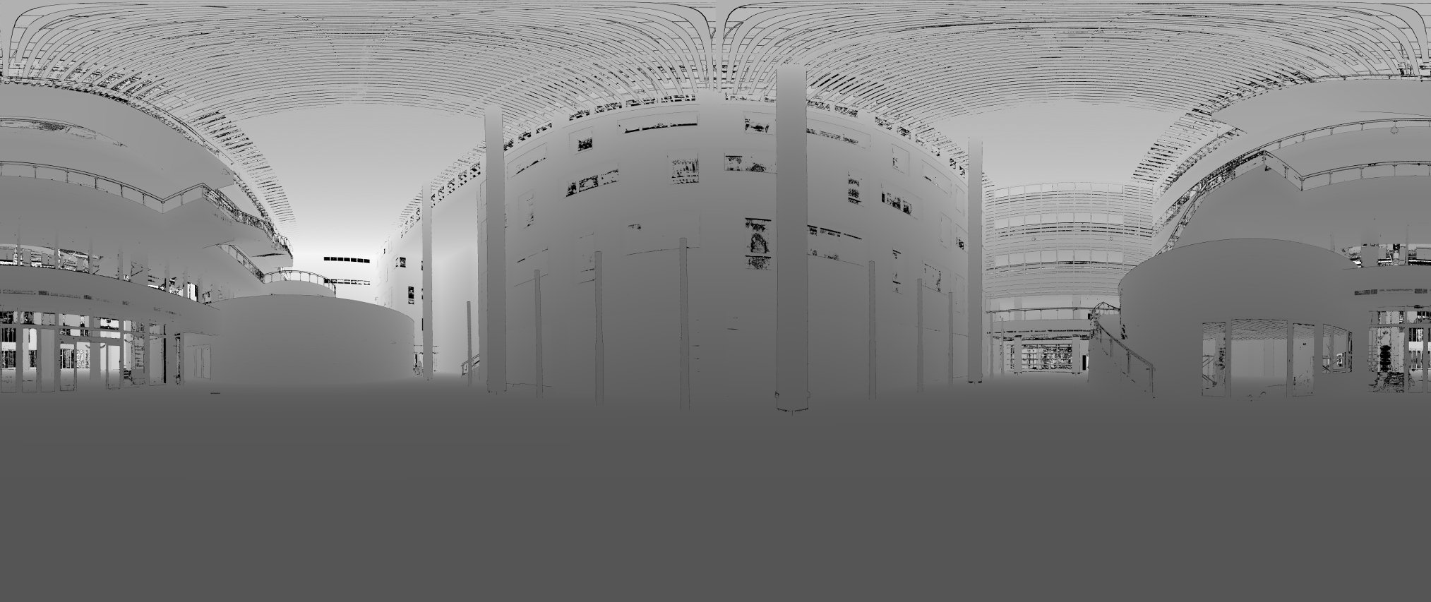
Below also a tool is available to convert such a depth image to a png. Figure 2 shows the depth image of the raw input scan. You may notice that there are many pixels (more than a million) which are black. For those pixels the scanner could not determine the distance.
We want to fill proper values into those missing pixels. Thus we take the information of the neighboring pixels into account. We use the same technique as Gaussian blurring, except that we apply this only to black error pixels. When we apply the Gaussian Kernel to an error pixel it also makes no sense to use this and other error pixels for the interpolation. We are thus omitting all error pixels during the convolution - and have to adjust the result for the omitted pixels, such that we get a properly normalized result again. See the implementation for details.
Also, only pixels which use at least 10% of the kernel weights are used in the convolution - otherwise the pixel will remain an error pixel. Thus bigger kernels with bigger standard deviation values are preferrable, but slow.
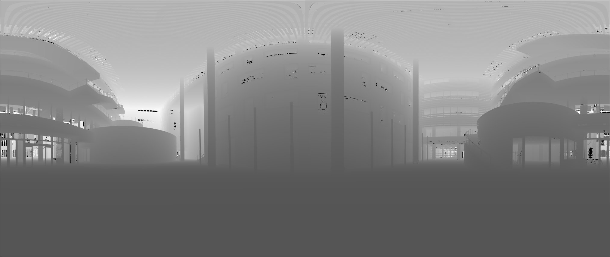
You are provided with the implementation for this algorithm (see below). This implementation is very slow. Your job is to make the execution as fast as possible, while still producing the correct result. Two solutions are provided: Figure 3 shows an interpolation with a small kernel (15x15), which only takes seconds to compute. You can use this for testing.
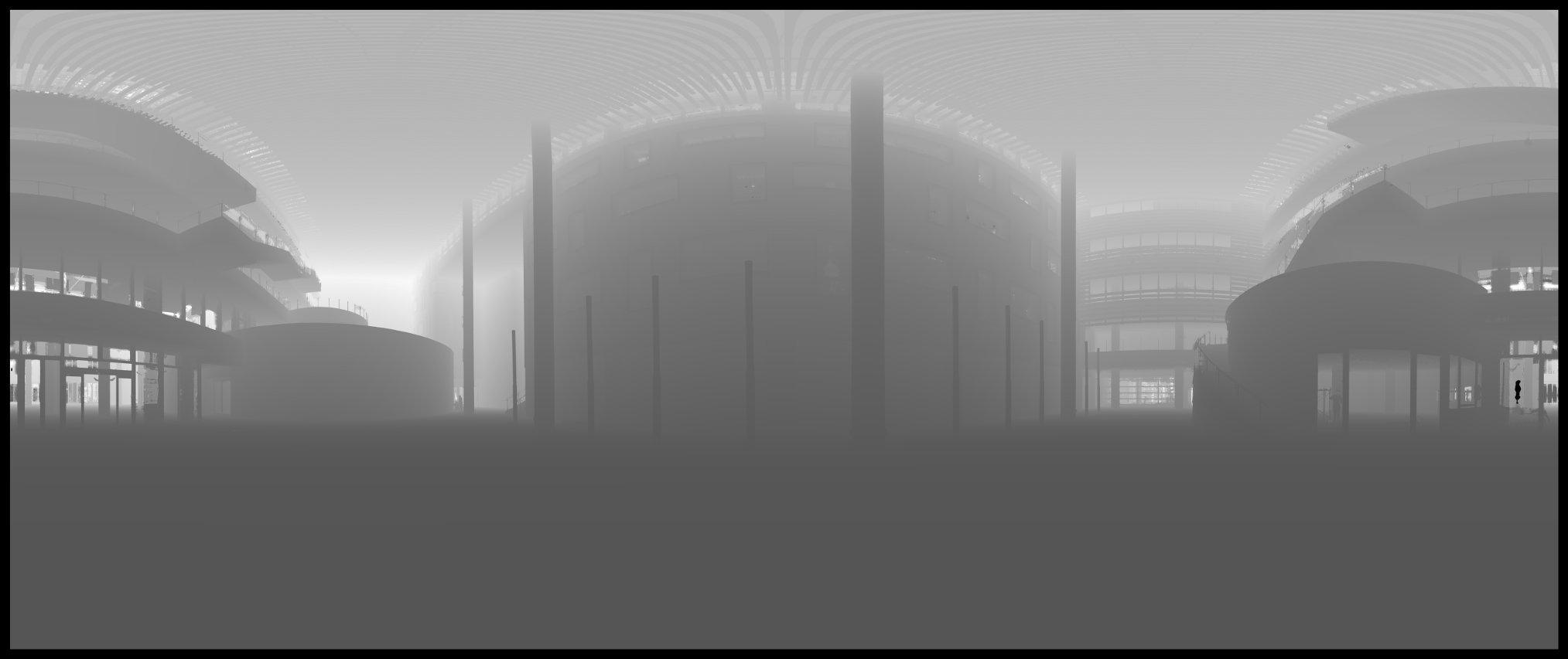
Figure 4 shows the depth map that in the end will be used for the competition. It was computed with a kernel size of 255x255 pixel and a standard deviation of 20.

Fig. 1: The scan of the lobby of the new SIST building in color. Full resolution (154MiB).

Fig. 2: The depth image of that scan capped at 60m. The darker the closer to the camera. Completely black pixels are error points. Full resolution (7MiB).

Fig. 3: Depth image where many of the error points have been removed by interpolation (kernel size 15, std. deviation 4). Computation time on the below system with the reference algorithm about 9 seconds. Full resolution (7MiB).

Fig. 4: Depth image where most of the error points have been removed by interpolation (kernel size 255, std. deviation 20). Computation time on the below system with the reference algorithm about 13 minutes. Full resolution (7MiB).
Notice that Figure 3 has still many error pixel remaining. This is because of the limited size of the kernel. Figure 4 has a bigger kernel (and standard deviation) and thus more error pixels are removed.
Also note that both interpolated images have a black "border" around the edges. This is because of the kernel size. A better implementation could still start from the edges, but would then have to perform extra checkings. Also such an improved implementation would need to take care of the fact that the image is 360 degree, the pixel next of the zeroth pixel of a line is the right-most pixel. But we ignore those details for this project.
Reference Program:
- interpolateFloatImg.cpp: Reference implementation.
Downloads:
- Input depth map: lobby.bin (660 MiB)
- Output depth map 255 20: intLobby_255_20.bin (660 MiB)
- Output depth map 15 4: intLobby_15_4.bin (660 MiB)
- Input depth map cropped: cropped.bin (3.8MiB)
- Output depth map cropped: croppedInt.bin (parameters: 277 10) (3.8MiB)
Tools:
- compareFloatImg.cpp: Compares two binary image files if they contain the same values, up to an epsilon provided as argument. This program will be used by the gradebot to check if your program computes the correct result. The epsilon used will be
0.0001 (0.1mm)0.002 (2mm). - floatImage2png.cpp: Takes a float depth image and creates an according png image for visualization. The maximum range has to be specified on the command line (if the actual max range in the image is smaller it will be used instead). Depends on libpng and png++ .
- Makefile for all three programs (for Mac - you will need to adjust the png++ location for your system - or comment out floatImage2png).
Task:
In the computer architecture lecture we have learned several techniques to make programs faster. Use them to implement the algorithm as fast as possible. You can change whatever you like - it is only important that your output is the same as the reference program. You may not use any specialized math library - SSE and openMP should be enough.Do NOT set the number of threads of openMP by hand - it will be set by the environment variable! Gradebot will punish you if you do.
The simplest approach is to take the reference implementation and start changing/ optimizing it.
Take care of what makes sense to optimize and what not. For example the reading and writing of the images is not part of the timing - so you do not need to change anything there.
Submission:
Check into gradebot:- interpolateFloatImg.cpp: Your fast implementation.
- Makefile: Your Makefile.
Grading
Gradebot will use a small map to test your program. If your output is incompatible you will receive 0 pts! Gradebot will show you the output of your program - keep it short! This way you will have a rough estimate how fast you are compared to the other students. But keep in mind that the gradebot is a shared resource, so those values might differ a lot.The gradebot checking will be implemented within this week.
Your program will be run on a 10 core (with HyperThreading 20) machine, using the 255, 20 parameters, running Ubuntu 14.04. The speed of each program will be noted.
The slowest 33 percentile and below will receive a score of 80%. The fastest 15 percentile will receive a score of 100%. All other programs will get a score that is linearly scaled between those values.
This project is only worth half of Project 1.1, 1.2, 2.1 or 2.2. (This project 11.11%, other (partial) projects: 22.22%).
Extra task (0 pts):
Let's make a small survey and see how different computer architectures influence the performance of the program. Please post the info of the performance of the reference program for the two kernel values in the according thread on piazza, like this:- Runtime 255 20: 753,752,010 microseconds
- Runtime 15 4: 9,381,568 microseconds
- CPU: Intel Core i7-4980HQ CPU @ 2.80GHz
- L1 $: 4x 32 KB data + 4x 32 KB instructions
- L2 $: 4 x 256 KB
- L3 $: 1 x 6MB
- Memory: 2 x 8 GB DDR3 1600 MHz